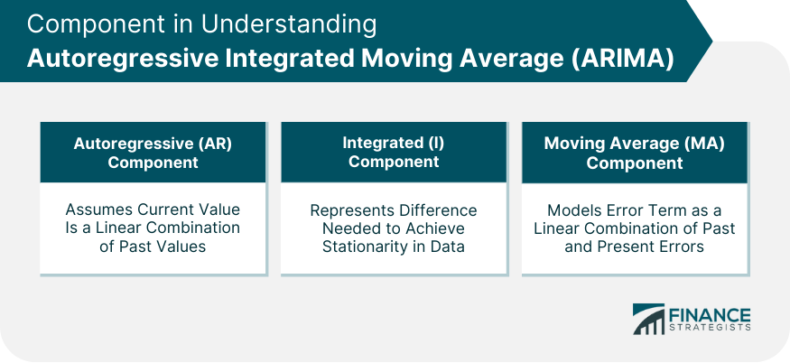
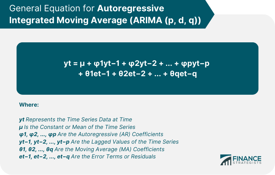
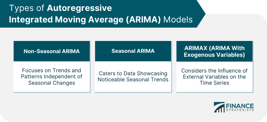
The ARIMA is a statistical modeling technique specifically designed for time series data analysis and forecasting. By combining autoregressive (AR) and moving average (MA) components with differencing integration (I), ARIMA models effectively capture trends, seasonality, cycles, and random walk in the data, making them particularly suitable for predicting economic and financial variables. ARIMA model is crucial in financial and econometric forecasting due to its ability to adapt to changes over time, accommodating a variety of structures in the temporal data. They provide insights into future events, enabling businesses to plan, strategize, and make informed decisions. Moreover, ARIMA models' ability to capture the stochastic properties of many economic, financial, and natural phenomena makes them a valuable tool for understanding and predicting a broad range of time-series data. The ARIMA model is comprised of three key components: This component assumes that the current period’s value is a linear combination of its past values. It specifies the number of lags of Y to include in the model. The integration component represents the difference required to make the time series stationary, thus dealing with trends in the data. Essentially, it subtracts the previous period's value from the current period's value. The moving average part involves modeling the error term as a linear combination of error terms occurring contemporaneously and at various times in the past. The ARIMA model is typically represented as ARIMA(p, d, q), where: p stands for the number of autoregressive terms, d is the number of nonseasonal differences needed for stationarity, and q indicates the number of lagged forecast errors in the prediction equation. The mathematical equation for ARIMA is a combination of autoregressive and moving average models integrated with differencing to make the time series data stationary. The general equation for ARIMA(p, d, q) can be represented as: The model assumes that the time series is stationary, implying a constant mean, variance, and autocorrelation over time. If it is not, differencing is applied to achieve stationarity. Invertibility is another assumption, implying that the model's error terms can be expressed as a linear combination of current and past forecast errors. Tailored for time-series data void of seasonality, the Non-Seasonal ARIMA model primarily concentrates on deciphering trends and patterns that remain independent of seasonal fluctuations. This makes it suitable for data that exhibit consistent behavior throughout the year without being influenced by seasonal shifts. Contrasting the Non-Seasonal version, the Seasonal ARIMA model, often symbolized as ARIMA (p,d,q)(P, D, Q)m, caters specifically to time-series data that showcase noticeable seasonal trends. The added notation (P, D, Q)m signifies the autoregressive, differencing, and moving average components exclusive to the seasonal aspect of the model. Meanwhile, 'm' stands for the count of periods within each season, defining the pattern's cyclical nature. Expanding the utility of the traditional ARIMA, the ARIMA model with Exogenous Variables, commonly termed ARIMAX, accounts for the influence of external or exogenous variables on the time series. It transcends the model's standard practice of relying solely on past values of the series, integrating external variables to enhance prediction accuracy. Implementing ARIMA models involves several steps: The process starts with the identification of the ARIMA model, which involves deciding the values of p, d, and q. The second step is estimating the parameters for the model. The model uses maximum likelihood estimation or non-linear least-squares estimation. Finally, diagnostic checks are carried out on the residuals. If the residuals are correlated, the model may be modified to improve its accuracy. ARIMA is widely used in predicting stock market prices. The model can analyze past stock prices and forecast future values, providing valuable insights for investors and traders. ARIMA is also applied in predicting foreign exchange rates. The model takes into account past exchange rates to predict future rates, providing valuable data for international traders and investors. Central banks and other economic entities use ARIMA models to predict inflation rates. These predictions are critical for setting monetary policy and other economic strategies. One challenge in using ARIMA models is identifying the correct order of differencing and the right number of AR and MA terms. Incorrect model identification can lead to inaccurate predictions. ARIMA models are limited by their reliance on stationarity and invertibility assumptions. Some time series data may not be made stationary or invertible, limiting the applicability of ARIMA models. The Autoregressive Integrated Moving Average (ARIMA) model, a powerful tool for time series data analysis, has distinct components: autoregressive, integrated, and moving average, that work together to capture the complex dynamics of temporal data. Its potency in forecasting is grounded on the assumptions of stationarity and invertibility. These assumptions necessitate a constant mean, variance, and autocorrelation over time and require that the model's error terms be expressible as a linear combination of past and current forecast errors. Various types of ARIMA models, including non-seasonal ARIMA, seasonal ARIMA, and ARIMA with exogenous variables, extend their applicability across diverse scenarios, enhancing its versatility. These features collectively make ARIMA a central pillar in the realm of financial and economic forecasting. As we navigate an increasingly data-driven world, the ability to understand and utilize ARIMA models can be a crucial asset.Definition of Autoregressive Integrated Moving Average (ARIMA)
Understanding ARIMA Model Components
Autoregressive (AR) Component
Integrated (I) Component
Moving Average (MA) Component
Mathematical Representation of ARIMA
Notations and Terminologies
Equation and Derivation
Assumptions of ARIMA Models
Stationarity
Invertibility
Different Types of ARIMA Models
Non-Seasonal ARIMA Model
Seasonal ARIMA Model
ARIMA Model Incorporating Exogenous Variables
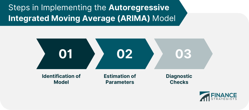
Steps in Implementing the ARIMA Model
Identification of Model
Estimation of Parameters
Diagnostic Checks
Application of ARIMA in Financial Forecasting
Stock Price Prediction
Foreign Exchange Rate Forecasting
Inflation Rate Prediction
Limitations and Challenges in ARIMA Modeling
Difficulties in Model Selection
Limitations Related to Stationarity and Invertibility
Final Thoughts
Autoregressive Integrated Moving Average (ARIMA) FAQs
ARIMA is used for time-series data analysis and forecasting, particularly in the fields of economics and finance. It can predict future values based on past and present data.
ARIMA models work by utilizing three components: Autoregressive, Integrated, and Moving Average. These components collectively allow the model to analyze different patterns and trends in the data and forecast future values.
The main assumptions of an ARIMA model are stationarity and invertibility. Stationarity means that the mean, variance, and autocorrelation of the time series data are constant over time. Invertibility refers to the condition where the model's error terms can be expressed as a linear combination of current and past forecast errors.
ARIMA models have limitations related to their stationarity and invertibility assumptions. They can be challenging to apply to non-stationary or non-invertible data. Furthermore, identifying the correct model parameters can be a difficult process.
With the advent of machine learning and big data, the application and effectiveness of ARIMA models are expected to improve. Machine learning can enhance the model's adaptability and learning capacity, while big data offers vast amounts of time-series data for ARIMA models to analyze and forecast.
True Tamplin is a published author, public speaker, CEO of UpDigital, and founder of Finance Strategists.
True is a Certified Educator in Personal Finance (CEPF®), author of The Handy Financial Ratios Guide, a member of the Society for Advancing Business Editing and Writing, contributes to his financial education site, Finance Strategists, and has spoken to various financial communities such as the CFA Institute, as well as university students like his Alma mater, Biola University, where he received a bachelor of science in business and data analytics.
To learn more about True, visit his personal website or view his author profiles on Amazon, Nasdaq and Forbes.